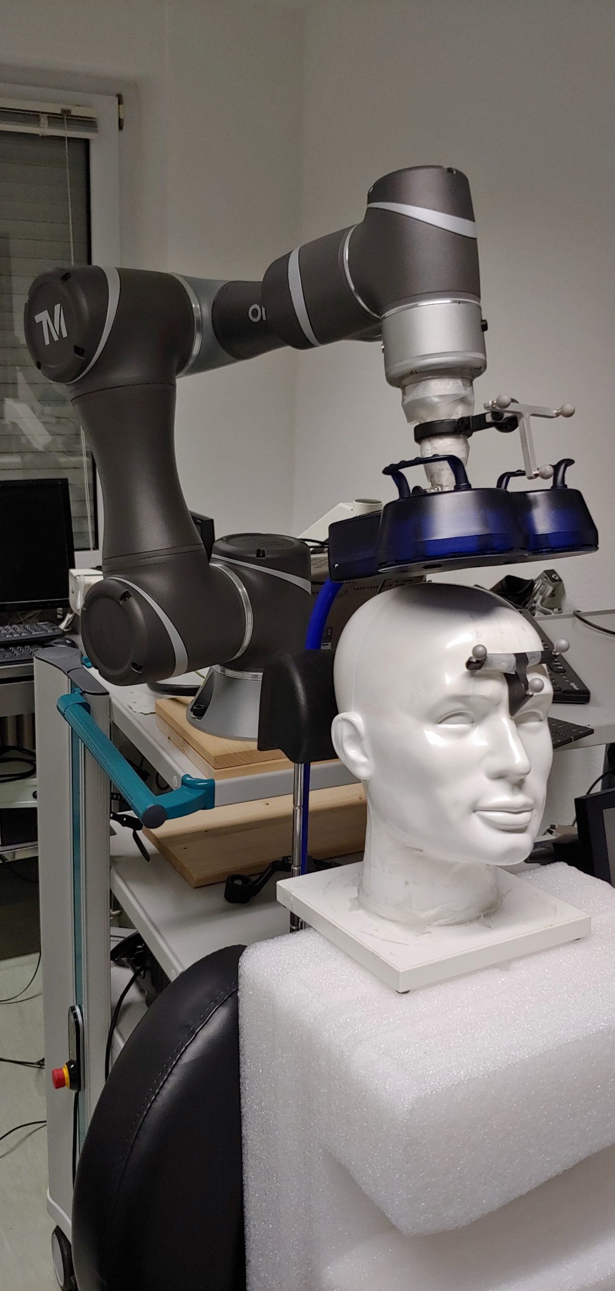
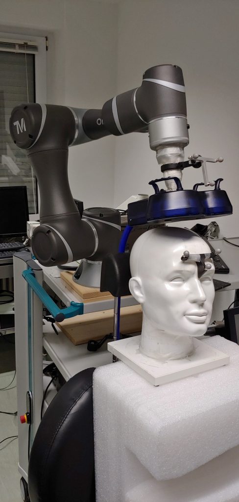
While working on my MD-thesis I got a bit sidetracked and ended up prototyping a robotic TMS-System.

What are you even talking about?

TMS stands for Transcranial Magnetic Stimulation — a fancy way of saying: Your brain gets stimulated with magnetic impulses. Using strong, pulsed magnetic fields, one can induce voltages in neurons, causing them to depolarize and fire an action potential. This in turn gets transmitted like any other action potential and allows e.g. to assess the integrity of neural pathways. Meaning, stimulating the brain results in twitches of the muscles associated with this part of the brain.
TMS has a wide range of uses. In research and is also used clinically as a therapy option for conditions like depression, whereas the reason for its application here is still discussed.
For further reading I recommand Siebner and Ziemann (2007) [german] or Rossini et al. (2015) (clinical application) as a starting point.

Why do you need a robotic system?

TMS relies heavily on stable coil placement — keeping the coil in the correct position relative to the head. Neuronavigation systems help with this by using 3D camera setups to track both the coil and the head, providing feedback whenever alignment begins to drift.

The challenge is maintaining that precise coil position over long sessions, especially if one has to manually hold the coil. And if the system already knows the coil’s location relative to the head, automation becomes an obvious next step.

When this project began, several commercial robotic solutions were already on the market. Nevertheless, a decision was made to develop an in-house system. An industry collaborator supported the effort by providing

• Software to extract 3D position data from the camera system,
• C# bindings to send position commands to a robot.

This led to the following system design — with the grey boxes representing the pre-supplied software components:

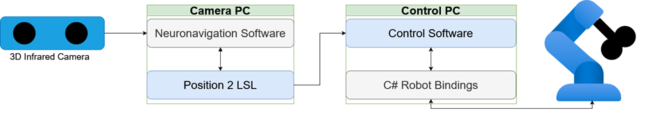
It was far from an ideal setup, but constraints around licensing, medical-grade software, and limited access to the camera PC left little room for alternatives. As it turned out, network latency was not the main bottleneck anyway.

Getting started felt deceptively straightforward. At the time I was not studying medical device engineering so with only limited robotics experience and mostly curiosity (plus some high-school math), the early steps were full of avoidable pitfalls. The initial plan was simple enough:

1. Solve the Inverse Kinematics,
2. Solve the Hand-Eye Calibration (align robot and camera coordinate systems),
3. Build the Control Logic (so the robot actually does what you want).

The inverse kinematics

The project began with what seemed like the most challenging task: implementing the robot’s inverse kinematics. (Ironically, this turned out not to be the difficult part.) This stage included a return to the Denavit–Hartenberg convention, which proved more helpful than expected.

Exploring an unfamiliar topic always brings a certain satisfaction, especially when it reveals an entire area one hadn’t encountered before. To experiment safely and avoid any risk during development, the robot model was added to a fork of the Robotics Toolbox for Python: https://github.com/Sebastian-Schuetz/robotics-toolbox-python

Surprisingly, the kinematic calculations themselves were relatively manageable. A complete solution for this specific robot already existed: https://repository.gatech.edu/server/api/core/bitstreams/e56759bc-92c8-43df-aa62-0dc47581459d/content

And someone provided code for the big brother of our robot and the required parameters could be taken from the manufacture: 

https://github.com/mc-capolei/python-Universal-robot-kinematics/blob/master/universal_robot_kinematics.py

This worked out quite nice. I play a bit with different implementations, because I was wondering about the atan2, but then found (Craig, 2005) who said, that this stabilizes the results. Most of the time in this phase was spent developing a deeper understanding of the underlying matrix operations, which ultimately made the kinematics feel far less mysterious.

Hand-Eye Calibration

With the kinematics in place, the next step was aligning the robot’s position with the camera coordinate system. The complication was that the neuronavigation software does not provide a fixed, absolute world frame. Instead, it defines the coordinate system relative to the participant’s head — specifically using anatomical landmarks between the ears and along the nasion–ear line.

Since heads inevitably move during long sessions, this creates a mismatch (e.g. if the coil is stationary):

• The target position on the head stays the same in the head coordinate system, while the coil position changes
• In the camera system the head moves, but the coil position stays the same

Luckily, this relative change is something we can work with — once we solve the infamous Hand-Eye problem

The Hand-Eye Problem (also called sensor–actuator calibration) is classic robotics homework:
How do you translate what the camera “sees” into movements the robot can actually perform?

Mathematically, it boils down to solving a simple-looking transformation equation:

A highly studied special (and simplified) case of this problem is:

First formulated (as far as I know) in this form by Tsai and Lenz (1989). A thorough technical overview is provided in (Furrer et al., 2018). In essence, once A and B are known, X can be estimated by recording multiple paired poses and solving an optimization problem that yields the transformation between the camera and robot coordinate systems.

Of course I am not the first to realize this, and there are a lot of solutions for solving equation (2):

• Dual Quaternions (Daniilidis, 1999)
• The Kronecker Product (Shah, 2013)
• And severel others

From earlier robot motion tests, a basic sequence of manipulator movements was already available. These included ±45° rotations around the Z and Y axes, smaller rotations around X, and simple translations along each coordinate axis. The initial pattern included individual motions such as:

Rotation around Z: +- 45°
Rotation around Y: +- 45°
Rotation around X: +-15°
Translation in X: +10 cm (and return)
Translation in Y: +10 cm (and return)
Translation in Z: +10 cm (and return)
Translation in X, Y, Z + 5 cm and Rotation around X, Y, C +15° (and return, all combined)

Reading more about this, I learned, that more elaborate strategies exist for getting the best poses to feed into the optimizer, here are some suggestions:

Tsai and Lenz (1989)
– Maximize rotation between poses
– Minimize the distance from the target to the camera of the tracking system
– Minimize the translation between poses
– Use redundant poses
– Have a star pattern

Or from Wan and Song (2000):
– Use a grid in the XY plane with randomized z heights and rotations
– (I needed to limit the angles here, because otherwise the coil would collide with the robot)

After testing various combinations of pose-generation strategies and solving methods, the best results came from pairing the simple pose set with the Kronecker-product approach by Shah (2013), implemented here: https://github.com/eayvali/Pose-Estimation-for-Sensor-Calibration
This combination consistently produced the highest precision.

The next question was how to quantify that precision?
For that I made use of the adapter I had designed for the coil. The design was a split design, with two metal rods, which would provide the strength and allignment, while a zip tie was used for rapid removal for manual operation. This is the cross section view:

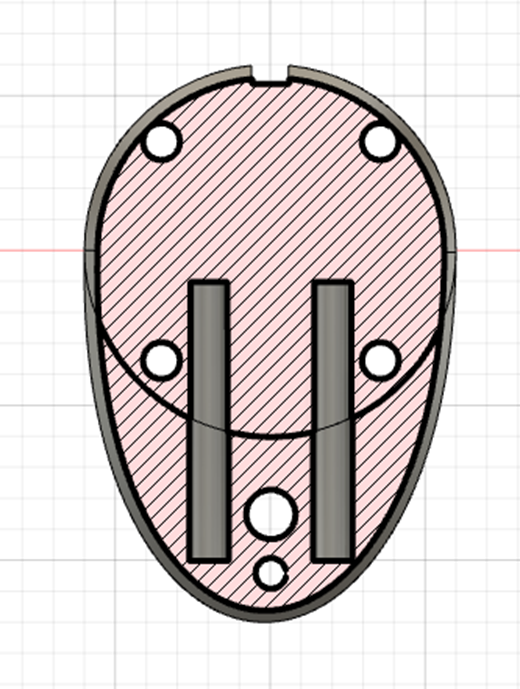
By adding a metal pin between the two components we could offset the coil by that diameter. I used a 7mm precission ground rod, because I had one on hand.
By inserting the pin, rerunning the calibration procedure, and comparing the translation components of the resulting transformation matrices, it was possible to evaluate how close each calibration result came to the expected 7 mm shift. The solution with the translation difference closest to 7 mm was considered the most accurate.

Building the Control Logic

After doing the ground work, the control system now ties everything together and is actually quite simple. The system works as follows:

1. Get Position from Robot and Camera
2. Calculate movement between current coil position and goal position on the head
3. Transform calculated move to robot coordinate system
4. Check this movement
5. Perform movement

For checking the movement I added a few safety considerations, mainly in regard the the following points:
Speed
Dont let the robot go to fast, I went with conservative settings, based on the manufacturers recommendations

Pose Selection
When solving the inverse kinematics, there are often multiple solutions on how a robot can reach one pose, for this robot, depending on the position, there can be up to 8 different poses that robot could take (Keating & Cowan, 2014)

Some of the eight possible IK solutions are clearly better suited than others—especially when a participant’s head is nearby—so I first defined a preferred pose (pose 2), which aligns best with the system’s mechanical design.
Among the remaining valid options, the robot selects the pose requiring the smallest angular change from its current configuration. Any pose demanding excessive joint motion is rejected outright: more than 30° in the shoulder or elbow joints (θ₁–θ₃), more than 50° in the wrist joints (θ₄–θ₆), or more than 100° of total joint movement (treated like a Manhattan-distance threshold).
To prevent jitter from camera noise, commands that would move the robot less than 1 mm or rotate it less than 0.5° are suppressed, while movements larger than 10 cm are blocked to ensure that participants can safely move away from the robot if needed.
Poses that would only be reachable using joint values outside legal limits are also discarded.
I had planned to add full collision detection—both between robot links (using the available STL model) and between the robot and the participant’s head—but did not have time to implement it. Even without this, the system was able to track head movements quite reliably. The main remaining limitation came from the C# bindings, which queued robot commands without allowing interruptions, resulting in a slow update rate of 1 Hz.

Grid Stimulation

Now, this is nice, but with a working tracking system one could do sooo much more. for example one could automate the detection of the stimulation point. To lay the groundwork for this we (myself and a bachelor student) implemented a way to project a grid on the head and stimulate on those points. For this to work we need

• A model or representation of the head.
• A coordinate system.
• A way to match real-world and virtual world.

Matching the real world and our model

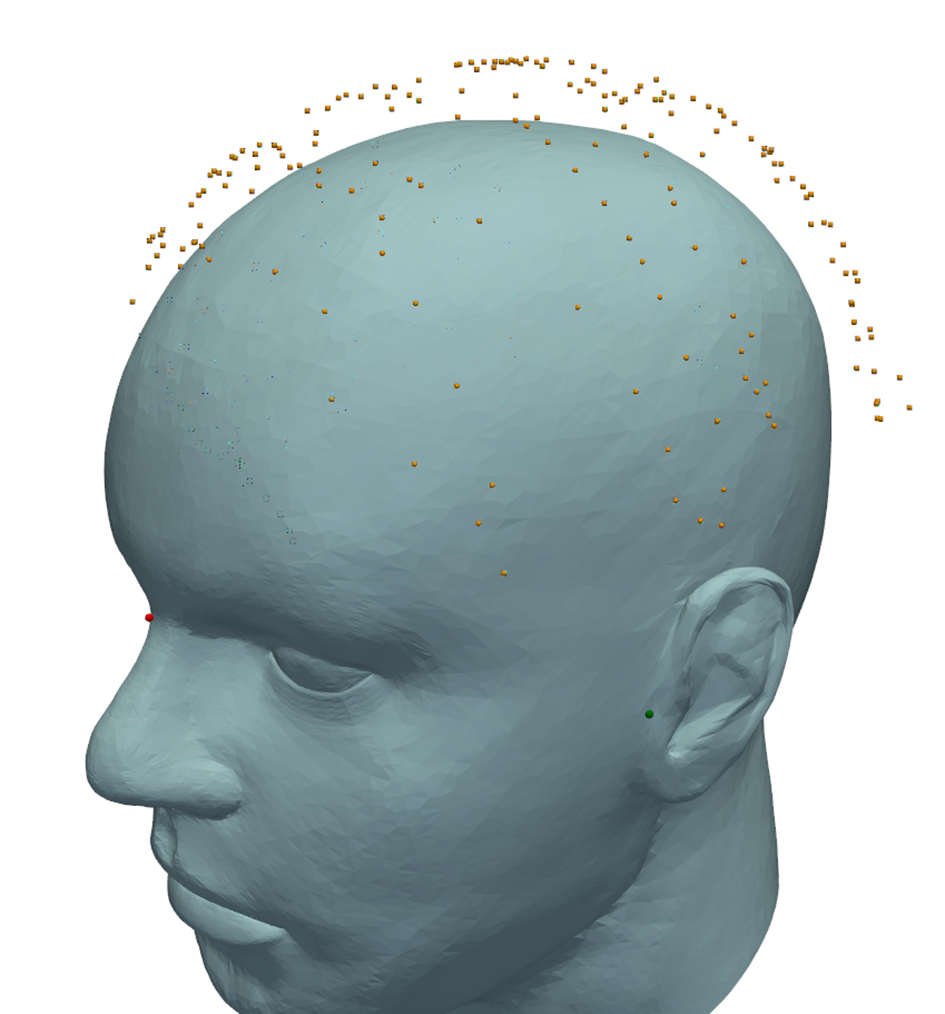
We borrowed some approaches from the neuronavigation software: Mainly defining a a head-centered coordinate frame from three anatomical landmarks: the nasion and the left and right preauricular points. And picking up a number of points from the participants scalp, more on that later. Corresponding points on the STL head model were located by manual inspection — a tedious process of searching, clicking and testing — but once the matches were found the alignment proceeded straightforwardly.

1. Scale the STL model to match the measured inter-aural (ear-to-ear) distance.
2. Translate the model so the left-ear landmark coincides with the measured left ear.
3. Rotate the model to align the ear positions (implemented as translate-to-origin → rotate → translate-back because PyVista does not support arbitrary rotation centres).
4. Rotate the nasion into place relative to the ears’ midpoint vector.

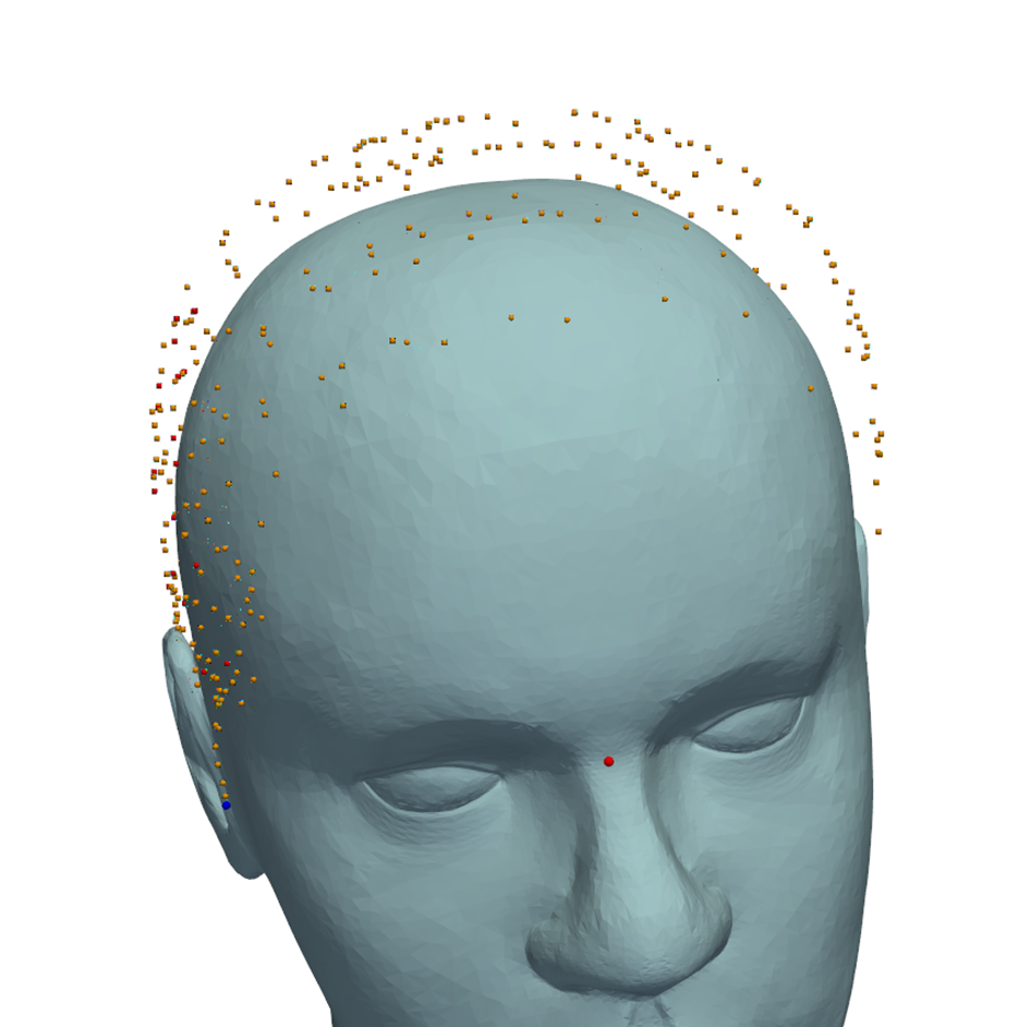
This produced a coarse but usable alignment. Note that scalp thickness (hair + cap, roughly 0.7 cm) caused the measured scalp points to be offset from the STL surface; nevertheless the aligned model correctly indicates the nasion and left-ear locations.

Mapping the grid to the real head surface

As one can guess, this is where the points from the scalp come in, but let me guide you throught the process on step at a time:

1. User defines the center point with pointer.
2. Create a planar grid (imaginary sphere tangent at center of the grid), 20 cm from the center of the coordinate origin
3. Map grid to the head.
4. Measure the actual distances on the head.
5. Scale grid accordingly and remap.

Obviously we thought about other ways too, but this ended up working so well, that we stuck with it. So, getting the point in the middle of the grid is the easy part, but how do we know how to position the grid tangent to the head surface?
Here the scalp points come in, that were recorded previously. Using open3d one can estimate normal vectors for a point cloud, which works pretty good:

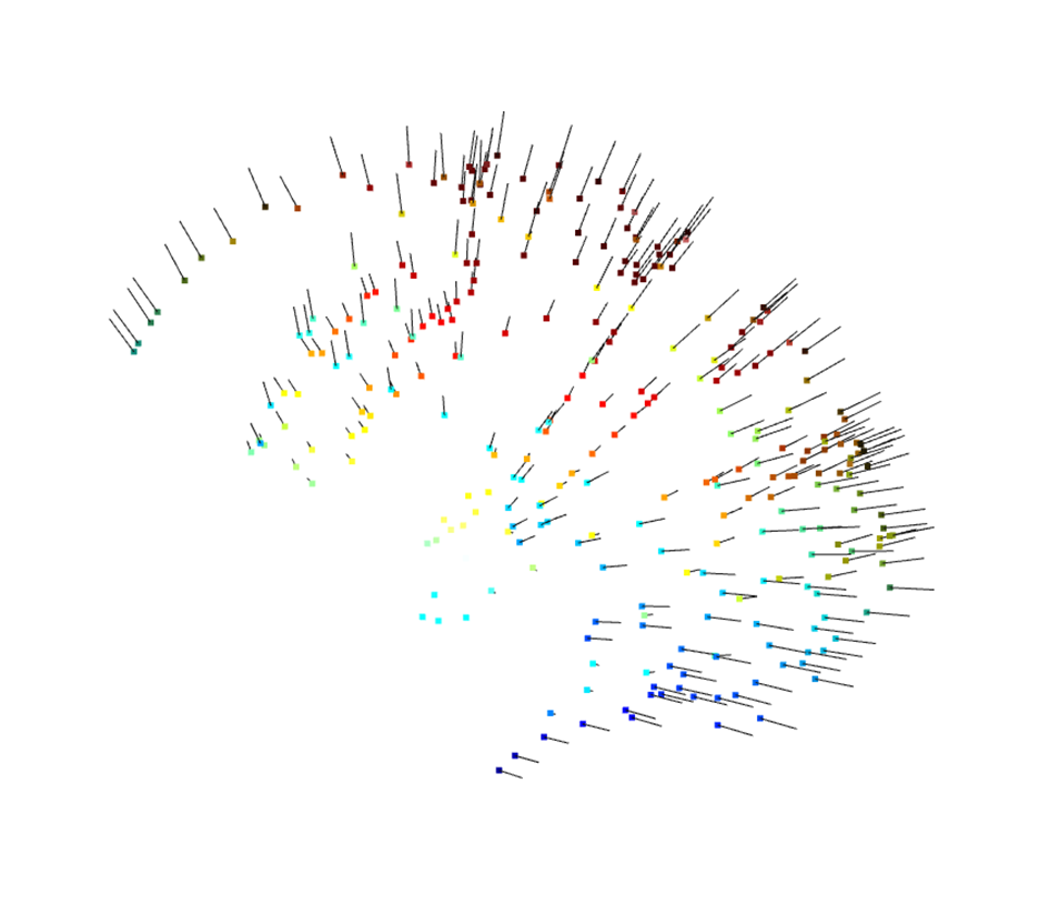
From here it is a simple matter of finding the points in the point cloud closest to the point selected by the user and average the normal vectors for the three closest points. This is the normal vector for the middle of the grid. From here, for each of the points in the grid, we went as follows:

1. Project a line from the coordinate origin through the grid point.
2. Find the three points closest to the line
3. Calculated the intersection of the line with the triangle plane for the position
4. Averaged the three normal vectors of the points for a stable orientation for the pose

This gives the position and pose tangential to the head surface. While not yet correctly rotated for the coil, we are getting there. The final step is measuring and scaling the grid to match the grid we actually want. This is also a simple process:

• Measured horizontal and vertical distances between neighboring points.
• Averaged them (approximate but practical).
• Calculated scaling factor.
• Regenerated a better-sized grid.
• Project from this new grid onto the head

The process can be seen here. In green there is the generation grid, which is tangent to the head surface. In red, one can see the grid, which was projected onto the scalp.

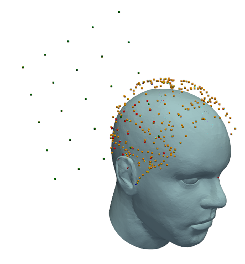
As one can see, the projected red points nicely follow the contour outlined by the scalp points

In order to compensate for the placement, we also added the option to rotate the generation grid.

Coil poses for stimulation

When performing TMS, the coil is tangential to the head surface, but often rotatet around the surface normal vector. To generate the desired rotation, we are going to modify the pose information we have now and build a rotation matrix for each point, which is easy, given, that we have the normal vector

1. Normal Vector = from scalp at each point.
2. Cross Normal with Z-axis → vector 1 (tangential).
3. Cross Normal with vector 1 → vector 2 (also tangential, orthogonal to vector 1).
4. Build a rotation matrix from Normal, vector1, vector2.

Voila, now we could just apply a final rotation matrix to the poses, (e.g., to make the coil 45° to the central sulcus/fissure), and done!

Lessons learned

Looking back, prototyping the robotic TMS system during my MD thesis became a formative experience—one that ultimately pushed me toward studying medical device engineering. I stumbled into nearly every classic robotics pitfall, from integration bottlenecks to opaque hardware interfaces, and I quickly realized how much engineering understanding I was missing. In hindsight, several lessons stand out. First, never underestimate the time and complexity required to integrate multiple subsystems; getting hardware, software, and control logic to cooperate is almost always slower than expected. Second, I learned not to let limited or poorly designed interfaces dictate my approach—next time, I would bypass the restrictive queued command implementation and communicate with the robot more directly. The same applies to the vision system: only later did I discover that the camera documentation actually included guidelines for designing custom markers, something I could have leveraged early on by simply 3D-printing my own.

Sources

Craig, J. J. (2005). Introduction to Robotics.

Daniilidis, K. (1999). Hand-eye calibration using dual quaternions. The International Journal of Robotics Research, 18(3), 286-298.

Furrer, F., Fehr, M., Novkovic, T., Sommer, H., Gilitschenski, I., & Siegwart, R. (2018). Evaluation of combined time-offset estimation and hand-eye calibration on robotic datasets. Paper presented at the Field and Service Robotics.

Keating, R., & Cowan, N. J. (2014). M.E. 530.646 UR5 Inverse Kinematics.

Rossini, P. M., Burke, D., Chen, R., Cohen, L. G., Daskalakis, Z., Di Iorio, R., . . . Ziemann, U. (2015). Non-invasive electrical and magnetic stimulation of the brain, spinal cord, roots and peripheral nerves: Basic principles and procedures for routine clinical and research application. An updated report from an I.F.C.N. Committee. Clin Neurophysiol, 126(6), 1071-1107. doi:10.1016/j.clinph.2015.02.001

Shah, M. (2013). Solving the robot-world/hand-eye calibration problem using the Kronecker product. Journal of Mechanisms and Robotics, 5(3), 031007.

Siebner, H. R., & Ziemann, U. (2007). Das TMS-Buch: Handbuch der transkraniellen Magnetstimulation: Springer-Verlag.

Tsai, R. Y., & Lenz, R. K. (1989). A new technique for fully autonomous and efficient 3D robotics hand/eye calibration. IEEE Transactions on Robotics and Automation, 5(3), 345-358. doi:10.1109/70.34770

Wan, F., & Song, C. (2020). Flange-Based Hand-Eye Calibration Using a 3D Camera With High Resolution, Accuracy, and Frame Rate. Front Robot AI, 7, 65. doi:10.3389/frobt.2020.00065